Kubernetes Cost per Request: A Transparent Formula

Calculating the infrastructure cost per API request gives you a clear view of service efficiency. Total cluster spend alone cannot show whether an application became more expensive to run or served more users. As traffic shifts, a flat monthly bill might hide a degrading service, while a rising bill might reflect successful growth. You need a unit-economics measure that connects cloud billing directly to business outcomes.

This process yields a working formula that calculates Kubernetes cost per request, combining direct workload expenses with a transparent share of shared cluster overhead. A change in this unit cost can signal an issue worth investigating. FinOps AI shows the cost side of this metric across AWS and Google Cloud (the request count comes from your own telemetry), alongside an approval-gated workflow that turns supported AWS findings into checked changes and rolls reversible ones back automatically if their check fails.

Before starting the calculation, define the prerequisites. You need a set service boundary, an agreed reporting window, a reliable request counter, and a deliberate choice between infrastructure-only and all-in costs.

Define the Unit and Its Scope

Distinguish between an incoming API request and a Kubernetes resource request. A Kubernetes CPU or memory request is a scheduling quantity. The scheduler uses this reservation to place Pods on available nodes, and this configured amount often differs from actual measured usage. An API request represents an incoming HTTP call or a completed business outcome, which is the event you will price financially.

Determine exactly what the denominator of your equation represents, whether that means attempted API requests, successful requests, or completed customer transactions. Count these events at the customer-facing service boundary, because treating every internal microservice hop as a separate user request inflates the denominator and creates an artificially low unit cost.

For comparable USD reporting across different periods, retain the underlying billing attributes. Keep the account or project, cloud region, billing window, and effective-cost basis identical when comparing rates over time.

For example, the FinOps Foundation Capability for Unit Economics lists cost per service request as one possible technical unit economics metric.

Use a Formula That Separates Direct and Shared Costs

A reliable calculation prevents cluster overhead from silently distorting application costs. The fully loaded infrastructure cost per request follows a specific formula. Take the service's direct infrastructure cost for the period, add its allocation share of any shared-cost pools, and divide that total by the chosen request count.

Direct costs include the CPU, memory, GPU, persistent storage, network egress, and load balancers attributed specifically to the service workload. Cluster-management charges, idle node capacity, and shared platform resources remain in distinct shared pools unless you directly provision them.

The OpenCost Specification separates workload costs, cluster idle costs, and cluster overhead in its cost model. It also says organizations can optionally distribute shared workload, cluster idle, and overhead costs among tenants.

When presenting the data, show the direct rate alongside the fully loaded rate. Dividing only the direct cost by the request count isolates the engineering choices made by the application owners. If you omit overhead from the calculation, label the result direct or workload-only rather than fully loaded.

Step 1: Choose a Workload Cost Basis

The cost basis you choose changes what the numerator means. No single approach answers every engineering and showback question, so select the basis that matches your organization's goals and technical constraints. The basis determines whether you charge for the resources a workload requests, the resources it consumes, or a combination of both.

Compare Requests, Actual Use, and Blended Models

Allocating CPU and memory cost based on configured resource requests shows the capacity a workload asks the cluster to reserve, assigning financial responsibility for over-provisioning directly to the service owner. When workloads request much more capacity than they use, request-based allocation captures that waste in the service's unit cost.

An alternative approach allocates cost based on the greater of configured requests or actual measured usage. This blended method accounts for reserved capacity while preventing usage spikes above the request limit from appearing cost-free, which is why OpenCost specifies this greater-of approach for CPU, memory, and GPU workload costs.

Actual-usage allocation relies strictly on measured consumption to highlight pure engineering efficiency, showing what the application consumed while executing its tasks. If you use this basis, keep the remaining idle capacity on the nodes visible in a separate pool or allocate it under a stated policy. Omitting idle capacity entirely produces an artificially low unit cost that fails to reflect the full expense of running the cluster.

Follow Your Provider’s Cost-Allocation Rules

For AWS EKS, split cost allocation data is available through legacy Cost and Usage Reports (CUR) and through CUR 2.0 with Data Exports. Cost Explorer does not include this data. AWS offers a resource-request option based on Kubernetes pod CPU and memory requests, and an Amazon Managed Service for Prometheus option that allocates Amazon EC2 costs using the higher of pod CPU and memory resource requests and actual utilization. With the resource-request option, only pods configured with CPU and memory requests receive split-cost data, while the Prometheus option requires all features to be enabled in AWS Organizations. For accelerated computing instances, only the resource-request option is supported. The AWS documentation on enabling split cost allocation data describes these choices.

Google Kubernetes Engine handles allocation differently, relying entirely on resource requests rather than measured consumption. The platform exports cluster and workload allocation data into detailed Cloud Billing exports in BigQuery, changing cost attribution for reporting purposes without altering the total GKE bill.

If you use third-party tools, verify their pricing source. OpenCost's Allocation API prices workloads at on-demand list prices (or a custom pricing sheet); its separate Cloud Costs API reads provider billing data. State clearly which cost basis your dashboard uses, because list-price allocation and provider-billed costs are not interchangeable. Tracking Kubernetes cost allocation by namespace provides a foundational layer for these calculations, giving you a defined boundary before applying shared costs.

Step 2: Allocate Shared Overhead Transparently

Shared costs require identifiable pools, as adding an unexplained markup percentage to every service creates friction between finance and engineering teams. Distributing these shared expenses based on logic and measurement builds trust in the final unit-cost metric.

Match Each Pool to a Cost Driver

Separate your shared expenses before applying any allocation weights. Create distinct pools for idle node capacity, resources reserved for system components, cluster-management fees, and shared ingress or observability infrastructure. Confirm that no cost appears in both a direct workload bucket and a shared pool.

Choose a distribution weight that reflects the underlying cost driver. A CPU or memory allocation share provides a logical basis for distributing compute overhead, while network bytes transferred may serve as a better distribution metric for a shared NAT gateway or ingress pool. Use equal splits across services only when leadership establishes equal allocation as an intentional internal policy.

Publish the exact calculation for each pool by showing the service weight divided by the total weight, multiplied by the pool cost. Transparency allows platform and finance teams to see why a service received its specific share of the overhead. The shares across all services should total exactly 100 percent for each fully distributed pool.

Keep Idle and Unallocated Costs Visible

Idle and platform costs should not disappear into a generic application charge. OpenCost provides mechanisms to retain idle cost in a dedicated allocation category or to distribute it proportionally across active workloads. GKE billing exports separate overhead into specific categories, labeling node resources set aside for system components and flagging resources not requested by workloads.

If you lack a defensible driver for distributing a specific shared cost, keep that balance in an unallocated platform-cost line. FinOps AI splits each node's cost across namespaces and workloads by their share of CPU and memory requests, and spreads system namespaces and DaemonSets across the other workloads. Its figures are therefore fully loaded, with no separate idle or platform-cost line; if your policy keeps an unallocated platform-cost line, calculate that line yourself.

Step 3: Divide by a Consistent Request Count

Align the numerator and denominator by dividing costs and request counts from the exact same service boundary over the identical reporting window.

For online API services, the request counter supplies the denominator. Decide early whether the unit means attempted requests or successfully completed outcomes. Keep attempted and failed requests visible in your monitoring tools even when your primary financial metric uses successful requests. Errors consume CPU, memory, and network bandwidth without delivering the intended business outcome, meaning a spike in error rates will drive up the cost per successful request.

The Prometheus Instrumentation documentation identifies query counts, errors, and latency as key metrics for online-serving systems. For those event counts, counters accumulate totals, and rate() gives their per-second rate of increase.

Maintain a strict boundary between infrastructure-only expenses and all-in service costs. If a service request also invokes a managed database, a third-party API, or an inference model, a Kubernetes-only numerator excludes those dependencies. Add external services only with an explicit scope and a defensible allocation method. Tracking AI spend alongside Kubernetes costs provides a broader view, provided you can correlate model charges with the service calls before merging them into a single per-request metric.

Step 4: Work Through a Hypothetical Example

Applying the formula to a concrete scenario demonstrates how the components interact. This analyst-created example uses hypothetical inputs to illustrate the arithmetic, rather than representing customer data, a provider rate, or an industry benchmark.

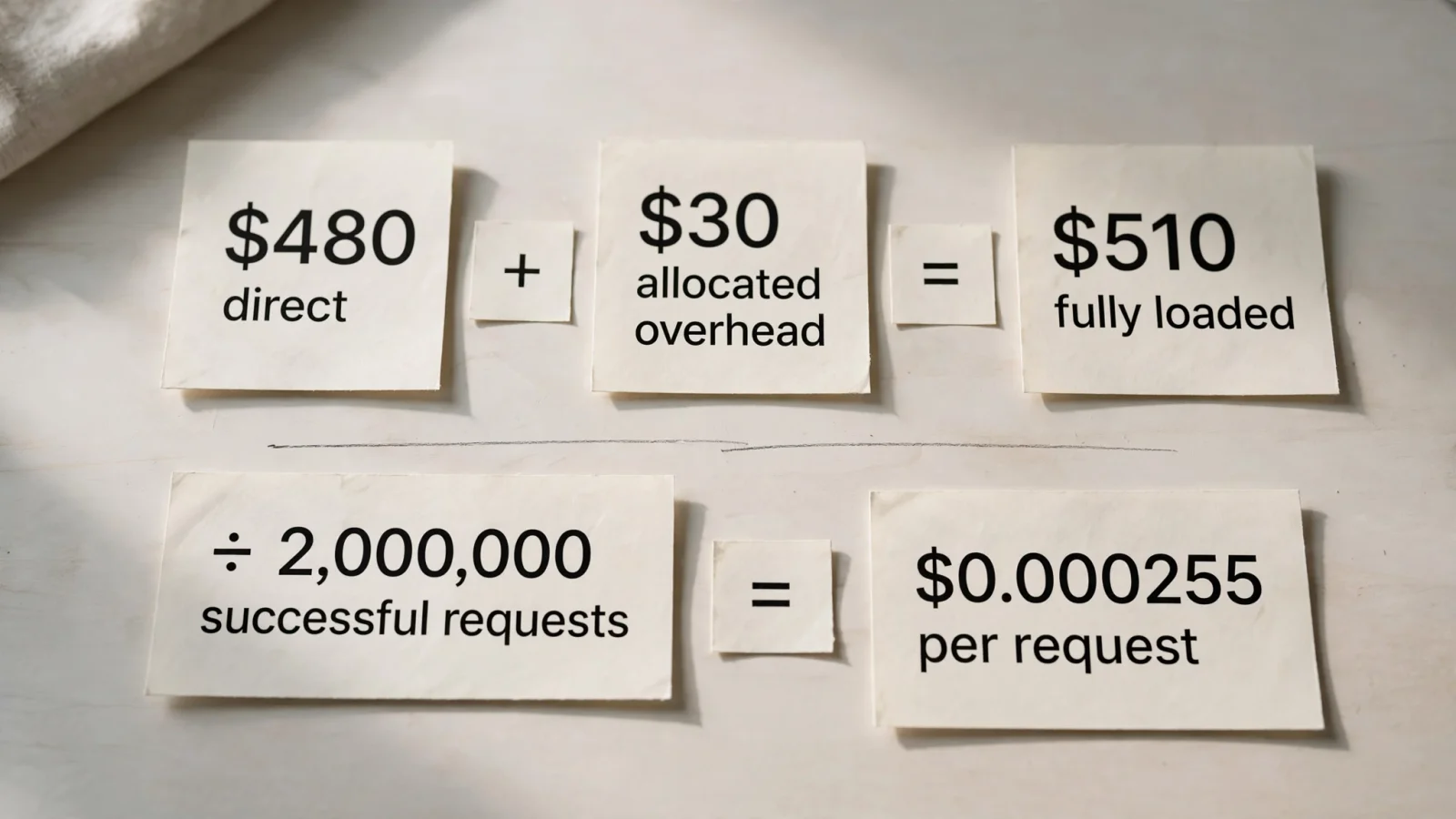
Assume a service incurs a direct infrastructure cost of $480 for the reporting period. The platform team maintains a shared cluster-cost pool totaling $120, and based on the chosen resource weight, the service takes a 25 percent share of that pool. During the same period, the service handles 2,000,000 successful requests.

1. Calculate the allocated overhead by multiplying the $120 shared pool by the 25 percent share, resulting in $30.
2. Determine the fully loaded service cost by adding the $480 direct cost to the $30 allocated overhead, yielding $510.
3. Divide the $510 fully loaded cost by the 2,000,000 successful requests.

The calculation yields $0.000255 per successful request, which translates to $0.255 per 1,000 successful requests.

Showing the direct-only rate provides helpful context for the engineering team. Dividing the $480 direct cost by the 2,000,000 requests produces a direct rate of $0.00024 per successful request, and displaying both numbers makes the burden of the shared overhead explicit. A different internal policy, such as retaining all idle capacity in a central platform budget rather than distributing it, would produce a different fully loaded rate.

Check the Rate Before Acting

A moving unit cost requires investigation rather than immediate automated intervention. Compare trends only when the service boundary, reporting period, billing basis, allocation policy, and request definition remain consistent.

When the rate spikes, inspect the underlying variables before assuming the application has become wasteful. Check the direct workload costs to see if CPU usage increased. Review the shared-pool shares to determine if another service scaled down, leaving this service with a larger percentage of the cluster overhead. Confirm the traffic volume, as a sudden drop in successful requests will inflate the unit cost even if infrastructure spending remains flat.

Watch for common calculation errors. You might confuse Kubernetes resource requests with HTTP API calls, resulting in a nonsensical denominator, or omit idle costs completely while labeling the result a fully loaded rate. Double-counting occurs when an organization adds a shared load balancer to both the direct service cost and the shared network pool. Mixing a 30-day billing window with a 28-day traffic window will also distort the final metric.

Pair your financial rate with reliability indicators. A lower cost per successful request provides no value if latency degrades or the service drops connections, as apparent savings might conceal a degraded user experience.

Use the unit metric to prioritize cost findings. A confirmed negative trend justifies dedicating engineering time to optimize Pod sizing, adjust scaling thresholds, or investigate application performance. The metric serves as a diagnostic tool that feeds into a broader workflow.

For supported AWS findings, FinOps AI uses an approval-first workflow. You apply guardrails: a production block you can set per account, and an optional workspace-wide cap on executions in a 24-hour window. When an owner or admin approves a change, the platform executes the remediation, records the action in an audit trail, and runs a post-action check. Reversible changes roll back automatically if that check fails. Google Cloud connections currently provide cost and usage visibility to support the analysis phase, though GCP remediation is not supported. This approach keeps cost-saving changes tied to the evidence behind them without handing unrestricted control to automation.

---

Discover how FinOps AI brings multi-cloud cost visibility and approval-gated AWS remediation into one workspace. Visit FinOps AI to explore the platform.