GPU Cost per Training Run: Build an All-In Model
Calculate GPU cost per training run with compute, storage, orchestration, shared overhead, and failed attempts—then compare experiments by model quality.
· 8 min read
Calculating an accurate GPU cost per training run starts with defining what constitutes an experiment, tracking failed attempts, isolating durable storage charges, and allocating shared platform overhead. Understanding the baseline unit economics of your machine learning workloads allows you to change infrastructure safely to save money. When a dashboard flags inefficient infrastructure, an approved, bounded AWS change with a post-action check provides a safer path forward. FinOps AI supplies this action layer, letting your team execute approved cost-saving remediations and roll back reversible actions automatically if the check fails.

Choose the Measurement Unit and Cost Basis
Defining exactly what you are measuring forms the foundation of any financial model. Because an experiment can span multiple executions, separating the logical trial from its physical attempts is the first structural decision in tracking expenses.
Start by defining an attempt as one specific job execution and an experiment as the broader logical trial, including initial attempts, failures, retries, and restarts. Assign every attempt a unique identifier in your tracking systems. If a scheduler overwrites the telemetry of a failed job with data from a successful retry, the financial impact of cluster instability disappears from your records. Losing that history removes your ability to measure the expense of wasted compute.
After defining the units, choose one of three cost bases to value the consumed resources:
- List price: Values resources at the public rate, isolating workload efficiency from procurement variables.
- Effective cost: Applies negotiated discounts, savings plans, and committed use agreements to the billing data.
- Marginal cost: Tracks only the direct charges added by launching a specific workload, ignoring sunk platform costs.
Applying one basis consistently across all comparisons prevents skewed data. Mixing list prices for one run and effective costs for another invalidates experiment comparisons. State clearly if you are reporting a net-cost basis by subtracting provider credits.
Count Every Billable Resource
Mapping every cloud charge generated by the attempt establishes an accurate total cost. Analyzing only the hourly accelerator rate overlooks the wider footprint billed by cloud providers.
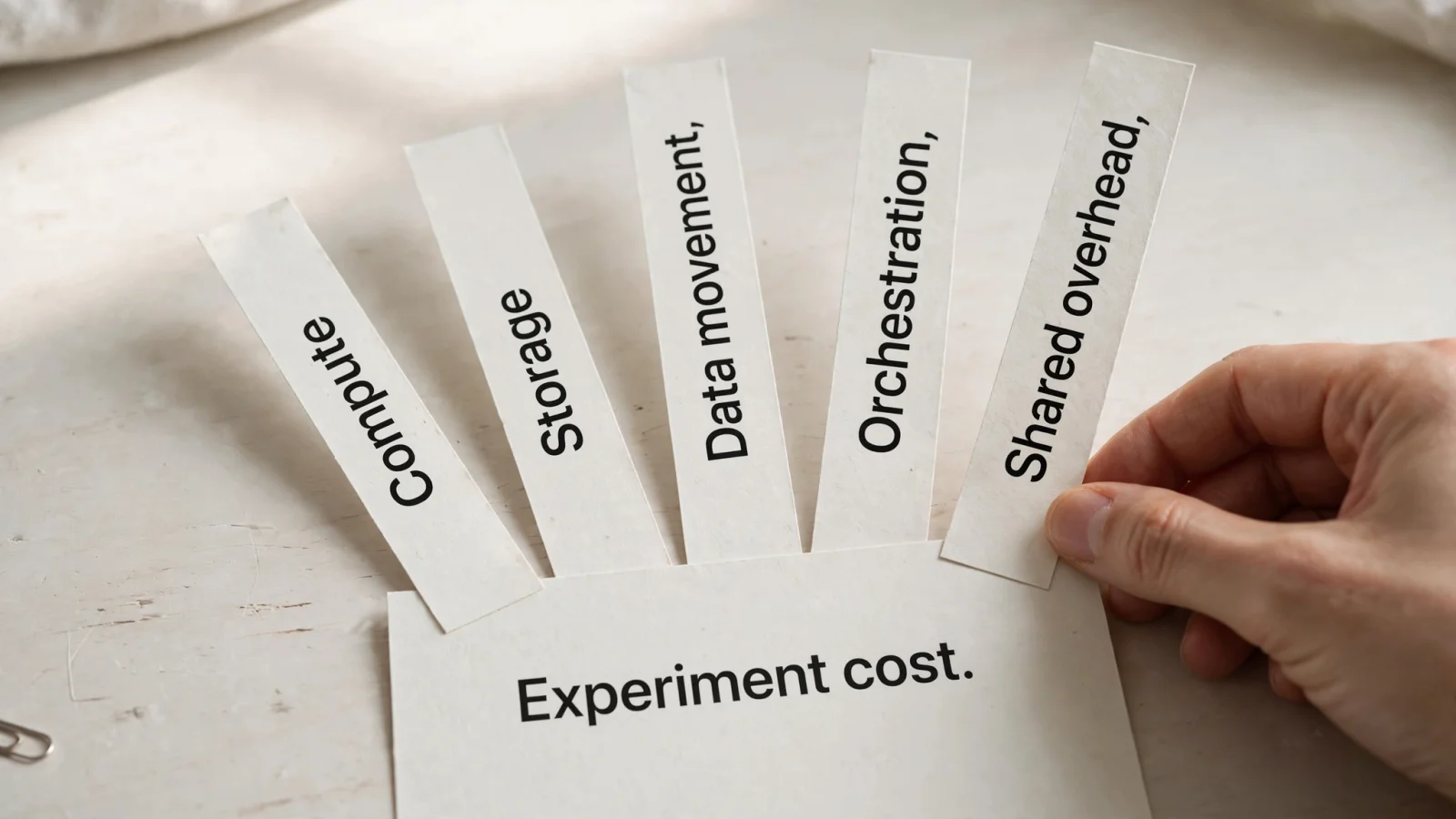
Compute charges extend beyond the physical accelerator to include CPU and memory when providers bill them separately. Use the provider's actual SKU structure to avoid adding component rates that the platform already bundles. For Compute Engine GPUs attached to general-purpose machine types such as N1, Google Cloud prices each GPU in addition to the machine type, so both line items belong in the financial model; for accelerator-optimized machine types such as A2, A3 and G2, the machine-type price already includes the GPUs.
Billable resources span the entire job lifecycle, from provisioning and container startup through data loading, the training loop, checkpointing, evaluation, and cluster teardown. Queue time remains distinct from provisioned time, though a running node waiting on data still incurs charges.
AWS On-Demand EC2 instances carry a 60-second minimum charge and bill by the second for time in the running state. That billing clock makes GPU utilization an efficiency signal rather than a direct substitute for billed instance time. If an expensive node sits idle for twenty minutes while reading a dataset into memory, the instance continues accumulating charges.
Storage components often outlive the compute resources. Scratch volumes, durable disks, model checkpoints, compiled artifacts, and any retained training data allocated to the run add to the total expense. Google Cloud documentation also confirms that durable disks remain billable while attached to a stopped or suspended instance, or when unattached to any VM.
Storage operations and data movement represent another significant expense. Pulling a massive dataset from object storage incurs request charges, and data-transfer charges when the bucket sits in a different region from the compute. Jobs that write large checkpoints frequently generate PUT requests that add measurable overhead.
Factoring in orchestration and platform resources accounts for the CPU and memory used by data loaders, schedulers, controllers, preprocessing tasks, evaluation scripts, and monitoring agents. Every failed, interrupted, or retried attempt belongs in the final total. If a job fails due to an out-of-memory error at hour ten, those ten hours of compute and storage remain part of the experiment expense.
Select a Shared-Cost Allocation Method
Because many machine learning workloads run on shared Kubernetes infrastructure, teams need to decide whether to allocate cluster overhead as marginal cost or fully loaded cost.
Marginal cost isolates the charges added strictly by the experiment, which helps evaluate incremental configuration changes. If an engineer adds a new parameter search, the marginal cost reveals the exact cash impact of that addition. Fully loaded cost assigns a portion of shared cluster fees, persistent datasets, and control plane overhead to the workload. This comprehensive view supports department chargeback and helps finance teams understand the broader economics of the AI initiative.
Running EKS or GKE introduces cluster-level considerations alongside the specific workload resources. Reviewing the applicable version, operating mode, and any active credits clarifies the final invoice.
Distribute shared charges across workloads using a single declared allocation driver, such as GPU-node time or requested CPU and memory limits. Overhead that is too complex to allocate accurately belongs in a separate report rather than being attributed to a specific job. For Kubernetes workloads, OpenCost measures and allocates cloud infrastructure and container costs, and its cost monitoring supports showback and chargeback. Dividing the total bucket cost of a shared dataset across multiple runs prevents double-counting, whereas multiplying the full amount by the number of jobs inflates the estimate.
Compare Allocation Strategies
Comparing the primary allocation strategies based on their operational focus helps determine which method fits your organization.
| Strategy | Included Components | Best Used For | Trade-offs |
|---|---|---|---|
| Marginal Cost | Direct compute, run-specific storage, direct egress | Evaluating single configuration changes and hyperparameter tuning | Ignores platform overhead, making total program cost seem artificially low |
| Fully Loaded Cost | Marginal cost + allocated shared cluster fees, durable dataset storage | Department chargeback and determining long-term ROI of an AI initiative | Requires complex driver definitions and constant reconciliation of shared assets |
| Accepted Result Cost | Total experiment spend (including all failed retries) ÷ number of successful models | Assessing framework stability, Spot instance viability, and overall pipeline efficiency | Heavily penalizes experimental architectures with naturally high failure rates |
Verify Cost Attribution Before Comparing
Connecting provider bills to specific model attempts relies on dependable telemetry. A consistent set of identifiers bridges the gap between engineering systems and cloud billing exports.
The necessary tracking fields include the experiment ID, unique attempt ID, model version, configuration version, and dataset snapshot. Additional details like the cloud account, region, cluster, namespace, resource SKU, and total GPU count provide infrastructure context. Logging timestamps, job status, failure reasons, the final validation metric, and the artifact location completes the data picture.
Applying tags or labels to billable resources wherever the provider supports them simplifies tracking. AWS cost-allocation tags demand specific activation for billing use. Confirming this activation and checking coverage ensure the resource tags appear in financial reports.
For AWS environments, the Cost and Usage Report (CUR) 2.0 adds resource-level IDs when INCLUDE_RESOURCES is enabled and split-cost allocation data when INCLUDE_SPLIT_COST_ALLOCATION_DATA is enabled; the split data can show how an EC2 instance's usage is allocated across containers.
When direct tags remain unavailable, joining billing records to job telemetry using resource IDs and timestamps creates a workable alternative. Any resulting allocation functions as a modeled estimate rather than a directly billed charge. Live cost dashboards remain estimates until reconciled against official billing exports. Google Cloud export delivery provides no latency guarantee, so immediate post-run calculations remain estimates until a final reconciliation against billing exports is possible.
FinOps AI brings AWS and Google Cloud cost visibility together with AI and Kubernetes spend monitoring. A shared workspace for multi-account spend, budgets, tag governance, and waste and risk findings with evidence and confidence scores highlights gaps in the attribution strategy. The platform team remains responsible for joining run-level billing data to model-training telemetry, while FinOps AI provides a governance framework for acting safely on AWS optimization opportunities.
Compare Experiments by Cost and Model Quality
Declaring the cheapest job the best one ignores performance requirements. A fast, inexpensive training run provides no value if the resulting model fails to meet the target accuracy.
Evaluating runs under a consistent validation protocol presents the total experiment cost directly alongside quality and completion status.
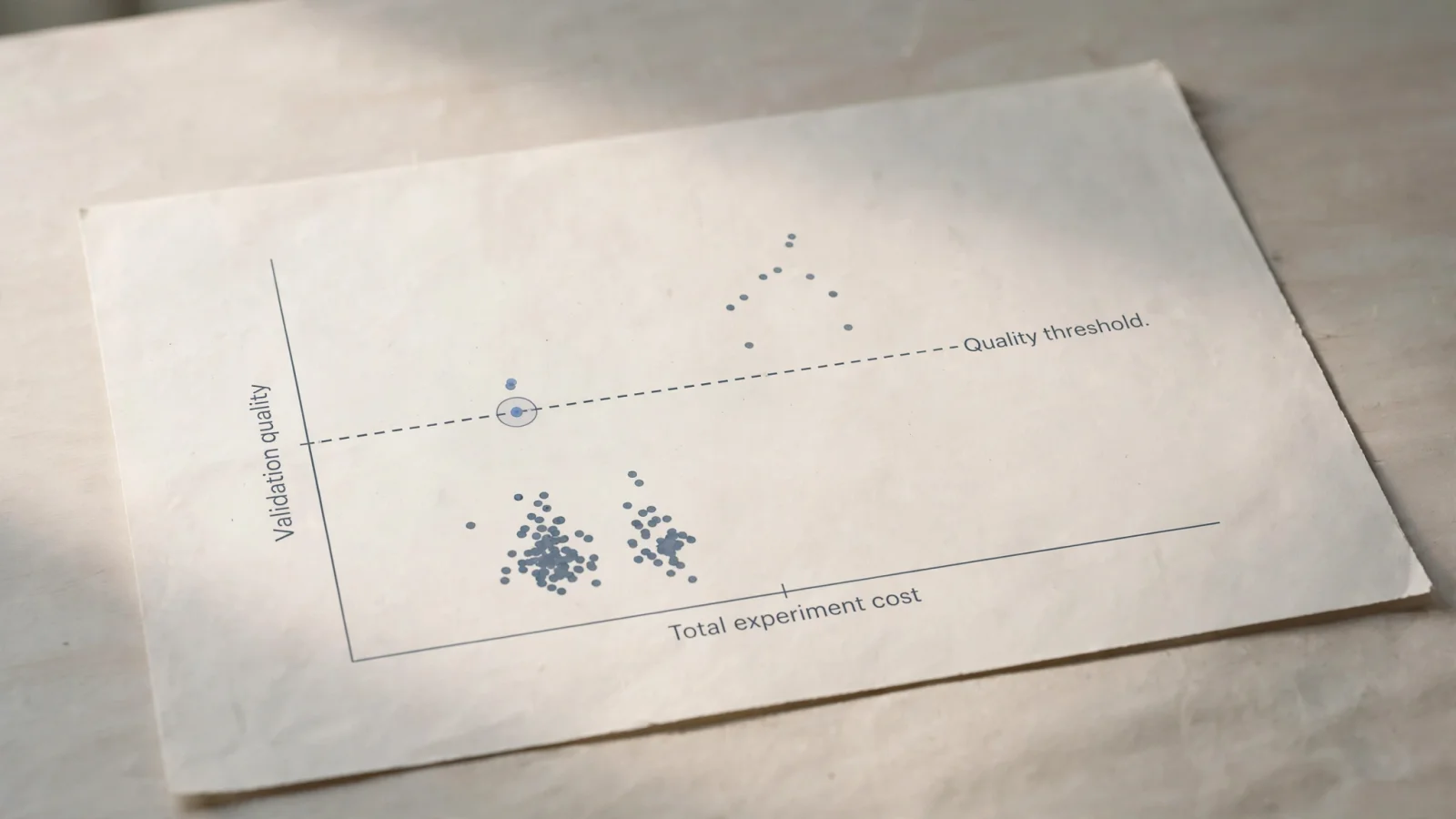
Tracking the expense per attempt, the total experiment investment across all attempts, and the elapsed time to reach a specified quality target provides a balanced evaluation. Calculating cost per accepted result requires care. For a portfolio of experiments, dividing the total charges across all experiments and attempts by the number of results that meet an agreed quality threshold reveals the true unit economics. Trials producing no accepted results still accumulate failed-run spend, which belongs in the final accounting.
A cost-versus-quality view identifies the lowest-cost configuration that crosses the quality threshold. Keeping inference or API charges outside this training denominator prevents skewed data, unless those charges genuinely belong to the experiment's execution. Monitoring Bedrock and Vertex AI spend within the same overarching cost view adds context, yet combining API inference costs with custom model training obscures unit economics.
Assessing Spot instances requires comparing the cost per accepted result rather than the advertised compute rate. Spot interruptions trigger checkpoint writes, node restarts, and checkpoint restores, which alter both elapsed time and total attempt expenses. Compute time spent between the last checkpoint and an interruption represents wasted effort that remains fully billed. Frequent interruptions can make a job running on Spot more expensive in total than one running on uninterrupted On-Demand instances. Relying on managed-job billing records for managed services provides better accuracy than assuming standalone EC2 billing behavior.
Apply the Model Through a Safe FinOps Workflow
Measurement creates value when it informs action. Reconciled cost and quality comparisons highlight infrastructure improvements, and follow-up reviews verify whether those changes shift experiment economics.
Unattached persistent disks often drive up experiment costs long after the instances shut down. Expensive accelerators sometimes sit idle for hours waiting for CPU-bound data loaders to finish preprocessing. Acting on these findings calls for a controlled environment.
FinOps AI governs AWS changes through typed, approval-gated actions. Account-level safety rules, a daily execution cap and approval by an owner or admin, which every change needs unless you turn on automatic execution for its type, help keep automation away from an active, heavily invested training job.
The platform runs a post-action check after a change executes and rolls reversible changes back automatically if that check fails. When an instance is stopped or an EBS volume or snapshot is deleted, the estimated saving is booked as pending and re-checked in AWS about seven days later; only changes that held count, and the figures are not reconciled against your cloud invoice.
The platform operates within clear boundaries. FinOps AI avoids calculating specific run-level telemetry for internal pipelines, tuning machine learning code, or providing GPU-specific compiler optimizations. For Google Cloud, the platform currently provides cost and usage visibility without active remediation.
With the run-level model and quality threshold explicit, teams can identify opportunities, build changes, route them through governed approval, and verify the financial outcome.
Turn cloud-cost findings into approved, guarded AWS changes with post-action checks, automatic rollback of reversible changes, and an audit trail of each change. Learn more at FinOps AI.
Sources
- GPU in addition to the machine type · cloud.google.com
- 60-second minimum · docs.aws.amazon.com
- durable disks remain billable · docs.cloud.google.com
- OpenCost · opencost.io
- Cost and Usage Report (CUR) 2.0 · docs.aws.amazon.com