GCP Egress Cost: Trace the Paths Behind Your Bill
Learn how to isolate GCP egress charges by service, region, and traffic path, then weigh savings against latency and architecture trade-offs.
· 12 min read
Managing precise Google Cloud egress costs requires comparing network architectures, evaluating billing data against traffic paths, and weighing infrastructure modifications against application latency. To support this investigation, FinOps AI provides multi-cloud cost visibility alongside AI and Kubernetes spend monitoring. While its core workflow focuses on turning AWS cost findings into approved, guarded infrastructure changes—checking each change afterward and rolling back reversible actions that fail verification—GCP remediation is not currently supported. For Google Cloud, you rely on this visibility to map the exact service driving a charge before altering a live route.
Treating routing options as architectural decisions means choosing between different transit networks, placement strategies, and caching models based on performance and budget. When you treat egress as a single line item, you miss the underlying infrastructure patterns that create those charges. Isolating each path allows you to evaluate specific architectural remedies without compromising system reliability.
Evaluate the Traffic Paths Shaping the Invoice
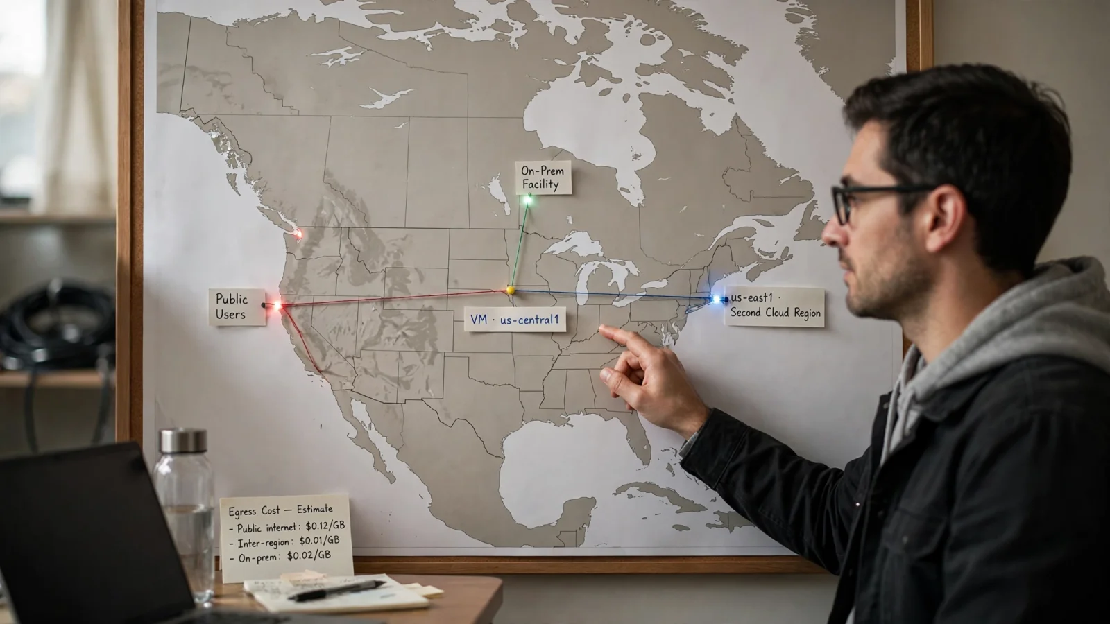
Google Cloud bills data leaving a resource based on destination, source location, and the specific service handling the transmission. Categorizing traffic according to Virtual Private Cloud pricing rules isolates the charges you need to investigate. Network transfers fall into several distinct tiers. Traffic moving within the same zone using internal IP addresses usually incurs no transfer charge, but crossing zones within the same region carries a specific fee. Data moving between regions on Google's backbone has another pricing structure, and data routed to the public internet or through Cloud Interconnect follows separate billing dimensions entirely. Assuming internal traffic is always free will lead to inaccurate forecasts.
Even within a single zone, addressing choices alter how Google Cloud meters the transfer. Routing between two virtual machines in the same zone using external IP addresses generates charges that private networking avoids. When instances communicate across zones within the same region, inter-zone data transfer rates apply to both sides of the connection. Distributed microservices accumulate these costs as their cross-zone communication scales.
Inter-region traffic follows a pricing scale based on the source and destination regions. Replicating databases or streaming logs between a primary region and a secondary recovery region routes data across Google's global fiber backbone. This dedicated backbone provides predictable performance and lower packet loss than public transit, yet each gigabyte transferred across regional boundaries adds inter-region network charges to your bill.
Cloud Interconnect provides private, high-capacity connections between on-premises data centers and Google Cloud Virtual Private Cloud networks. Dedicated Interconnect and Partner Interconnect charge for port connections and VLAN attachments alongside specialized outbound data-transfer rates. Classifying all traffic leaving Google Cloud as generic public internet egress obscures these purpose-built hybrid rates.
Inbound traffic generally carries no VPC network data-transfer charge. Services processing that incoming data may still bill for compute or inspection time. Every response your servers generate counts as outbound transfer and contributes to the total bytes billed. Pinpointing the cost requires identifying the exact origin service, the destination network, and the routing tier managing the connection.
Group the Billing Lines Behind the Spend
Cost investigations start in the billing export. Grouping charges by service and SKU prevents guessing which application is responsible.
Google Cloud's standard BigQuery export provides the baseline dimensions for this evaluation. Querying the table groups charges by service description and SKU, which you can then narrow by project and usage location. The detailed export adds resource-level cost data where available, tying specific virtual machines or storage buckets to the spend. To place GCP costs in a broader cloud context, FinOps AI's multi-cloud cost view shows GCP spend by service beside your AWS spend, to help prioritize which workloads to investigate first.
A structured BigQuery query against your billing export table isolates the top contributors to data transfer costs. Grouping by service.description, sku.description, and project.id clarifies whether your spend is driven by Compute Engine internet egress, Cloud Storage network operations, or inter-region replication. Adding usage_start_time windows lets you correlate billing surges with specific deployment events or application traffic spikes.
If location.location is a region or zone, the location.region field in the standard data export structure identifies the region where usage occurred. This standard export lacks resource-level cost data and external client IP fields. Billing location alone cannot show which resources served the data or whether those gigabytes went to users in Europe, mobile clients in Asia, or a third-party software provider.
Labels provide allocation context by mapping costs to specific applications. Missing historical labels mean that earlier spend lacks grouping context, because label-based allocation only begins from the moment you apply the metadata to the resource. Consistent tag governance ensures that future billing exports contain the information needed to group charges accurately. Combining these verified billing dimensions with network telemetry allows you to map the full path.
Auditing historical spend across unlabelled infrastructure requires relying on project boundaries and resource hierarchies to infer ownership. Establishing automated label policies across your deployment pipelines ensures that newly provisioned instances, buckets, and forwarding rules carry metadata directly into subsequent BigQuery billing records.
Evaluate Endpoints Using Network Telemetry
Billing data confirms how much a service charged, but it rarely names the exact downstream client. You need network telemetry to evaluate the source and destination endpoints driving the volume.
VPC Flow Logs record network flows sent from and received by VM instances, GKE nodes, and other VPC resources. These logs contain source and destination IPs, protocol types, port numbers, and endpoint metadata. Capturing external IPs provides geographic clues about the destination, while logs from GKE environments include specific pod and cluster details when the system identifies the endpoint.
Analyzing these flow records in Cloud Logging or BigQuery uncovers the communication patterns responsible for high transfer volumes. You can identify internal services passing uncompressed JSON payloads between subnets, pinpoint instances communicating across regional boundaries without using internal endpoints, and detect misconfigured services routing internal traffic across public IP addresses. Flow metadata in Kubernetes environments attributes cross-node network volume to specific workloads, namespaces, and pods.
VPC Flow Logs supports network forensics and analysis of network usage to optimize traffic expenses. Because it samples packets, it estimates total traffic from those samples. The system also includes geographic regions for external sources and destinations.
Telemetry carries its own financial impact. Google Cloud bills VPC Flow Logs to the project containing the reporting resource, and exporting high volumes of log data introduces additional ingestion and storage charges at the destination service. Filtering the log scope to specific subnets and estimating the volume prevents the investigation itself from generating secondary expenses.
Enable VPC Flow Logs selectively on subnets supporting high-spend workloads rather than globally across an entire VPC network. Setting sampling rates and aggregation intervals according to your diagnostic goals keeps telemetry volume manageable. After you identify the offending network path and implement a fix, adjust the sampling rate or disable flow logging on those subnets to minimize recurring overhead.

Match Each SKU to Its Architecture
Every data transfer SKU corresponds to a specific architectural choice. Matching the billed line item to the components handling the traffic lets you evaluate the available trade-offs.
Compute Engine and VPC traffic depend on the IP type, the zone, and the external route. A path leaving through a Cloud NAT gateway adds complexity. Cloud NAT preserves outbound data-transfer fees while listing NAT processing charges and outbound internet transfer as separate cost components. This structure means you pay for the gateway processing time, the bytes processed, and the resulting network data transfer out of the VPC.
Using Cloud NAT allows private instances to access external services without assigning public IP addresses to each virtual machine. Routing multi-gigabyte data exports or large container image downloads through a NAT gateway accumulates both the per-gigabyte NAT gateway processing fee and the standard VPC egress rate. For workloads communicating with supported Google APIs, configuring Private Google Access bypasses the NAT gateway entirely and routes traffic directly to Google services over internal IP paths.
Cloud Storage evaluations require comparing the bucket location with the location of the consuming service. Google Cloud distinguishes between internal data movement, specialty network routing, and general outbound internet transfer. A specific region is not automatically the same location as a multi-region boundary that happens to encompass it. Applications in a specific region reading from a multi-region bucket incur different transfer charges than applications reading from a strictly regional bucket in the same zone.
When an application hosted in a regional Compute Engine cluster frequently reads objects from a dual-region or multi-region bucket, those read operations cross storage placement boundaries. The billing engine meters the data retrieval according to cross-location storage transfer rules. Consolidating storage into a single region that matches your compute workload eliminates these transfer fees, though you must assess whether your disaster recovery plan still meets business requirements.
Cloud CDN shifts the evaluation from direct transfer rates to cache mechanics. Serving cacheable content through the edge network replaces direct Compute Engine or Cloud Storage transfer charges with CDN delivery rates. Non-cacheable responses bypassing the edge still incur standard data-transfer fees. The final CDN cost calculation incorporates cache egress, cache fill from the origin, cache lookups, and any storage-operation charges triggered by misses.
Origin infrastructure also plays a role in CDN financial outcomes. An edge node experiencing a cache miss fetches the requested object from the origin Compute Engine backend or Cloud Storage bucket, generating cache-fill traffic. A low cache-hit ratio due to rapidly changing content or short time-to-live settings causes the combined cost of cache-fill bandwidth, lookup requests, and backend processing to exceed the cost of serving the data directly.
Select a Mitigation for the Proven Path
Modifying a network cost requires changing a live application. Prioritize mitigations by testing how they affect user experience, latency, and reliability. Altering a high-volume route without evaluating performance trade-offs risks degrading the service to save a marginal amount.
On AWS, FinOps AI's approval-gated workflow checks each change after execution and rolls back reversible changes that fail that check; it does not test latency or reliability, so that testing stays with your team. GCP remediation is not currently supported: teams use FinOps AI's cost view to see which services drive the spend, then trace the paths with the billing export and flow logs described above and apply changes through their existing deployment controls.
Internet-facing traffic offers a choice between Network Service Tiers. The Premium Tier routes traffic across Google's global low-latency backbone, handing the data off to public internet service providers close to the user. The Standard Tier acts as a cost-oriented alternative that drops traffic onto public transit networks much closer to the Google Cloud region, subject to regional eligibility limits. Cloud CDN requires Premium Tier routing, making it necessary to test Standard Tier latency with representative users before switching a live production path.
Standard Tier routing suits workloads where network performance is secondary to operating cost. Asynchronous batch processing, non-critical background uploads, or regional back-office utilities fit this model well. Routing traffic over public transit networks introduces variability in packet transit times and increases vulnerability to internet congestion. Premium Tier remains the better choice for real-time web applications, financial transaction processing, and user-facing SaaS platforms where consistent latency directly impacts user retention.
Caching models require realistic hit-ratio estimates. The edge network shortens the physical path to users and serves cached responses faster than origin servers, but cache misses add cache-fill latency and incur the underlying processing fees. A CDN acts as a strong architectural choice for highly cacheable content reaching a distributed user base, rather than acting as a guaranteed cost reduction for dynamic payloads.
Analyze the cacheability of your payload headers before enabling a CDN. Static media assets, public software packages, and pre-rendered client bundles achieve high cache-hit ratios, making them ideal candidates for edge delivery. Personalized API responses, dynamic GraphQL endpoints, and real-time streaming data generate frequent cache misses. Optimizing the origin application often yields better financial and operational results for dynamic workloads.
Data reduction often proves safer than network reconfiguration. Compressing text payloads, batching API responses, and implementing aggressive client-side caching lowers total transfer bytes without altering VPC routing. Applying these changes at the application layer reduces the volume of data before it ever reaches the billing meter.
Enabling modern compression algorithms such as Gzip or Brotli on HTTP response headers significantly reduces the byte count of JSON payloads, HTML documents, and JavaScript bundles. Auditing microservice architectures for chatty polling loops and replacing them with event-driven notifications or WebSockets reduces repetitive data transfers across internal subnets and regional boundaries.

Validate Savings Against Production Requirements
Architectural changes require validation. A proposed network fix must address the specific SKU driving the charge while justifying the potential impact on system resilience. Evaluating mitigations works best using a structured decision matrix that maps current configurations to potential adjustments.
The decision matrix prioritizes these evaluations:
| Evaluated Path | Driving SKU or Service | Primary Architectural Trade-off | Verification and Safety Action |
|---|---|---|---|
| Internet-facing VM traffic | Direct Compute Engine outbound | Routing cost versus Standard Tier public transit latency. | Measure round-trip times across representative user locations before changing tiers on production load balancers. |
| Cross-region VM to VM | Inter-region VPC transfer | Zone co-location versus high-availability failure domain separation. | Verify that consolidating workloads into a single region maintains recovery time objectives and disaster recovery capabilities. |
| High-volume static assets | Cloud Storage or Compute direct | CDN cache delivery rates versus origin processing and cache-fill costs. | Audit response cache headers, calculate expected cache-hit ratios, and model total request lookup charges before routing traffic. |
| Internal application reads | Cloud Storage outbound | Regional bucket co-location versus multi-region geographic redundancy. | Confirm whether data compliance or regional durability standards permit moving objects from multi-region to regional buckets. |
| Private outbound requests | Cloud NAT gateway and egress | Secure gateway management versus per-gigabyte NAT processing fees. | Configure Private Google Access for internal subnets to route API traffic directly to Google services without passing through NAT. |
Validating the exact source and destination pricing before modeling the savings helps ensure accuracy. Charges vary based on the specific services, geographic locations, network tiers, and usage brackets. A heavily trafficked route reaching users in one continent carries a different unit price than an identical service reaching users in another. The Cloud CDN pricing structure adjusts charges based on the destination geography and the total monthly volume.
Volume brackets in Google Cloud network pricing mean that the effective unit cost per gigabyte decreases as monthly transfer milestones are reached. If your organization operates under a negotiated custom contract or committed use arrangement, your actual invoice rates will diverge from standard public list prices. Modeling cost reductions using public calculator rates without factoring in negotiated discounts can lead to distorted return-on-investment projections.
Checking the applicable SKU and your negotiated billing contract provides more accuracy than relying on a generalized estimate. Implementing the change in a representative testing environment lets you monitor application latency alongside the matched billing periods. This confirms the architecture supports your recovery objectives.
Adopt a phased canary approach when rolling out network adjustments in production. Migrate a small percentage of client traffic to a newly configured Standard Tier route or regional storage bucket while monitoring application error rates, response latencies, and downstream dependencies. Compare BigQuery billing export records for the canary project against baseline historical data. This verifies that the targeted SKU reflects the expected cost reduction without shifting expenses onto unexpected secondary services.
Turning cost findings into secure infrastructure changes requires a platform built for platform engineering and SRE teams. FinOps AI provides multi-cloud cost and usage visibility, along with AI and Kubernetes spend monitoring. Its approval-gated agentic remediation workflow currently supports AWS, keeping humans in control of infrastructure modifications, checking changes afterward, and rolling back reversible changes that fail verification. While GCP remediation is not currently supported, teams use FinOps AI to see GCP spend by service beside AWS, investigate egress with the methods above, and apply changes through their own controls. See how FinOps AI approves AWS changes, checks each result and rolls back reversible changes at getfinops.cloud.
Sources
- Virtual Private Cloud pricing · cloud.google.com
- standard data export structure · docs.cloud.google.com
- VPC Flow Logs · docs.cloud.google.com
- Cloud CDN pricing · cloud.google.com