GCP Billing Export Analysis: Find Cost Drivers
Use GCP billing exports to explain project and service cost variance, uncover attribution gaps, and route evidence-backed findings to owners.
· 9 min read

A cost variance is useful only when its comparison basis is clear and someone can investigate the underlying infrastructure change. Finding a spike in cloud spend often leads to a dashboard alert that sits unassigned because the data lacks context. Effective cloud financial management requires moving past alerts to create a record of accountable changes. In an AWS environment, the FinOps AI platform turns cost findings into approval-gated, guarded changes that it then executes. Teams review an audit trail, and the system automatically rolls back reversible changes if their post-action check fails.
Google Cloud requires a different approach. FinOps AI currently provides cost and usage visibility for Google Cloud rather than direct remediation. Investigating those costs requires querying the underlying data directly. A thorough GCP billing export analysis explains project and service cost variance, uncovers attribution gaps, and routes evidence-backed findings to the correct resource owners. Extracting that evidence means understanding exactly what the exported data covers, setting a reliable comparison baseline, and preserving ownership labels as you aggregate the charges.

Choose an Export and Verify Its Coverage
Export granularity and data coverage define the limits of a cost analysis. Before writing a query to explain a variance, determine which BigQuery export table you are targeting and whether its update schedule supports your investigation.
Standard for Trends, Detailed for Resource Questions
Google Cloud provides two primary data streams for analyzing consumption. The Standard usage cost export tracks broad project, service, and SKU trends. It includes fields for the billing account, invoice month, project identifiers, service names, location data, usage quantities, and credit adjustments. It does not provide resource-level cost tracking, which keeps the table size manageable and query costs predictable. The standard table typically follows the gcp_billing_export_v1_<BILLING_ACCOUNT_ID> naming pattern.
The Detailed usage cost export includes all the standard fields alongside resource-level data for supported services. This level of granularity helps teams identify the costs associated with a specific Compute Engine instance. Accordingly, Google recommends using the standard export for cost trends and the detailed export for resource-level cost analysis. Querying the detailed export can cost more than querying the standard export, because BigQuery charges for the data read by each query.
| Export Type | Use Case | Table Naming Pattern | Resource-Level Data |
|---|---|---|---|
| Standard | Project, service, and SKU trends | gcp_billing_export_v1_<ID> | No |
| Detailed | Specific instance or cluster investigations | gcp_billing_export_resource_v1_<ID> | Yes (for supported services) |
Check Freshness, Backfill, and Gaps
A recent partial period can look like a sudden drop in spend because not all service usage data is available right away. Since services report usage at varying intervals, Cloud Billing exports data to BigQuery at regular intervals without delivery or latency guarantees, so a recent total can omit late-reported usage.
Initial data backfill depends on your chosen dataset location. For a first-time standard or detailed export into a US multi-region BigQuery dataset, the system provides retroactive usage-cost data starting from the beginning of the previous month. This initial backfill can take up to five days to complete, meaning an export enabled on October 4 will include backfilled data starting September 1. A supported regional dataset operates differently, as it collects data from the enablement date forward rather than backfilling historical usage.
Disabling and re-enabling an export creates a permanent gap for the period the export was turned off. Changing the destination dataset also leaves historical data behind. Dataset locations are fixed at creation, making it important to select a location that aligns with your backfill requirements and regional compliance rules early in the process.

Set a Fair Comparison Baseline
Defining the exact time window determines what your comparison explains. You are either explaining a finalized billed amount or tracking consumption over a specific period, and those two concepts require different date fields.
Use Invoice Month or Usage Time Deliberately
For invoice reconciliation and finance reporting, rely on the invoice.month field formatted as YYYYMM. This field maps every line item to the specific finalized bill it appeared on. Analysts inspect the cost_type field alongside the invoice month because invoices include taxes, adjustments, and rounding errors that fall outside actual resource consumption.
For operational consumption trends, use the usage timestamps provided in the export to track when the infrastructure was running.
The dates associated with usage and invoicing often differ. For example, late-reported usage from the end of January can appear on the February invoice, and the invoice.month field identifies the month of the invoice containing each cost line item. Comparing an incomplete month-to-date consumption period against a full finalized invoice month creates a misleading variance, so it helps to state your comparison basis clearly before presenting a finding to an engineering team.
Separate Usage, Cost, and Credits
Explaining why a number changed requires isolating consumption from pricing, which the export separates into distinct fields. The cost field reflects the applicable consumption model and includes negotiated discounts where applicable, while cost_at_list shows the baseline price before those negotiated discounts.
Credits exist as a nested field within the export row. Calculating the net cost requires adding the summed credit amounts to the initial cost field. A lower net bill might reflect a new committed use discount or a promotional credit rather than a reduction in resource consumption.
Retain currency identifiers in your grouping logic when combining multiple billing accounts, as summing different currencies as a single numerical value produces invalid reporting. If you are reconciling a full invoice month rather than isolating operational changes, retaining all tax, adjustment, and rounding rows keeps the totals accurate.
Trace Variance by Project, Service, and SKU
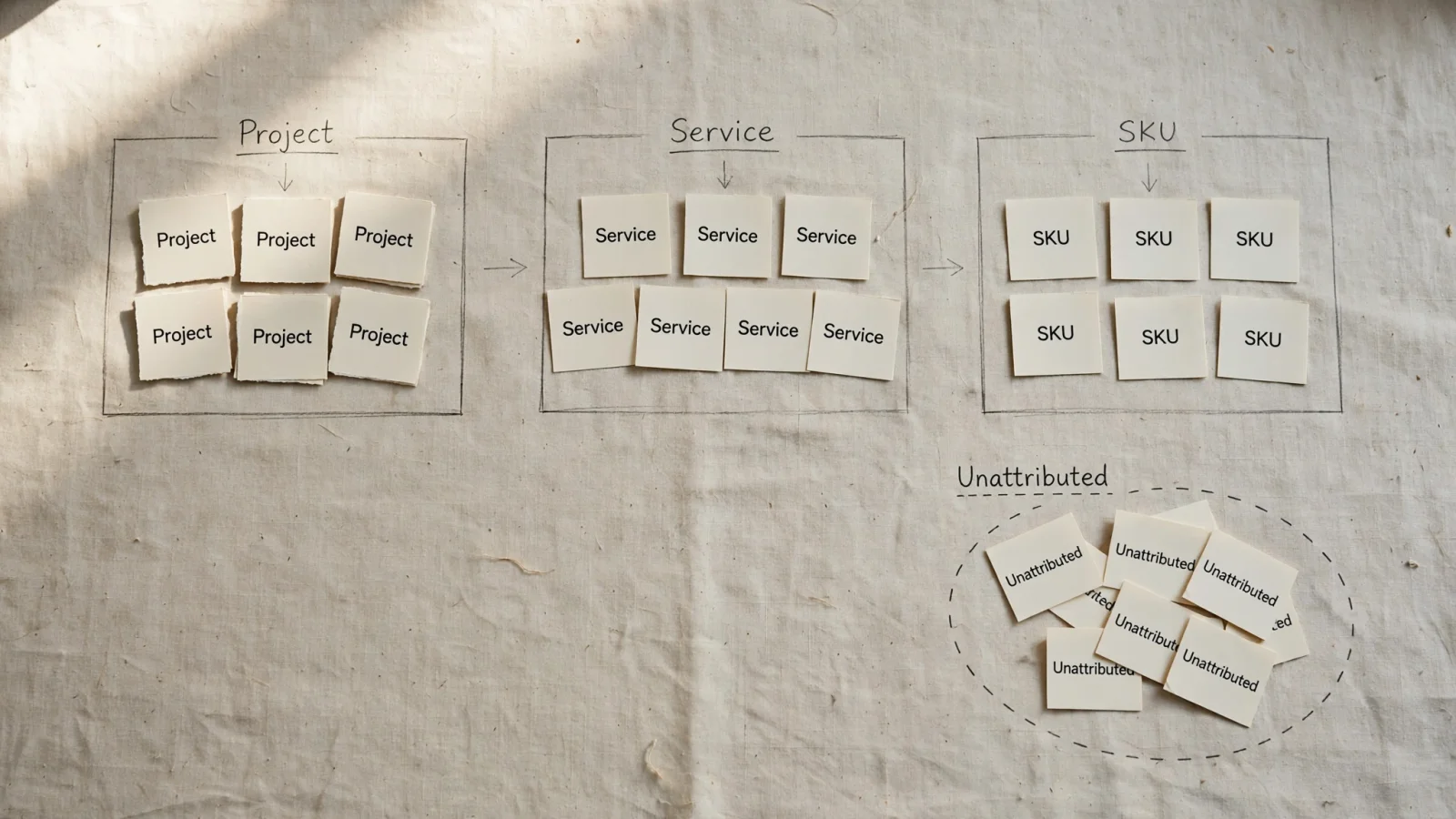
Investigating a spike begins at the project level, moves to the specific service, and narrows down to the billing SKU. FinOps AI supports this discovery phase through a unified multi-cloud cost view that shows AWS and Google Cloud cost by account and marks daily spikes on the cost chart, alongside waste and risk findings with evidence and a confidence score. Once you spot an area to investigate, running a billing-export query in BigQuery isolates the exact drivers.
This SQL example compares two invoice months at the project, service, and SKU level. It calculates the regular cost after credits and extracts a specific project owner label. Pass the @prior_month and @current_month parameters as YYYYMM strings.
WITH line_items AS (
  SELECT
    invoice.month AS invoice_month,
    project.id AS project_id,
    project.name AS project_name,
    (
      SELECT l.value
      FROM UNNEST(project.labels) AS l
      WHERE l.key = 'owner'
      LIMIT 1
    ) AS project_owner,
    service.description AS service,
    sku.id AS sku_id,
    sku.description AS sku_description,
    location.region AS region,
    currency,
    usage.amount AS usage_amount,
    usage.unit AS usage_unit,
    cost_type,
    cost,
    IFNULL(
      (SELECT SUM(c.amount) FROM UNNEST(credits) AS c),
      0
    ) AS credit_amount
  FROM
    `BILLING_PROJECT.DATASET.gcp_billing_export_v1_BILLING_ACCOUNT`
  WHERE
    invoice.month IN (@prior_month, @current_month)
)
SELECT
  project_id,
  project_name,
  project_owner,
  service,
  sku_id,
  sku_description,
  region,
  currency,
  usage_unit,
  SUM(IF(invoice_month = @prior_month, cost + credit_amount, 0))
    AS prior_net_cost,
  SUM(IF(invoice_month = @current_month, cost + credit_amount, 0))
    AS current_net_cost,
  SUM(IF(invoice_month = @current_month, cost + credit_amount, 0))
    - SUM(IF(invoice_month = @prior_month, cost + credit_amount, 0))
    AS cost_delta,
  SUM(IF(invoice_month = @prior_month, usage_amount, 0))
    AS prior_usage,
  SUM(IF(invoice_month = @current_month, usage_amount, 0))
    AS current_usage
FROM
  line_items
WHERE
  cost_type = 'regular'
GROUP BY
  project_id,
  project_name,
  project_owner,
  service,
  sku_id,
  sku_description,
  region,
  currency,
  usage_unit
ORDER BY
  ABS(cost_delta) DESC;
Filtering for cost_type = 'regular' isolates standard usage charges for an operational variance analysis. Because this filter excludes taxes and adjustments, the result will not match a finalized finance invoice perfectly. To reconcile a full invoice, remove the filter and categorize the non-regular cost types in a separate column.
Read the results by comparing the usage delta against the cost delta. If the net cost changed but the usage volume remained steady for a comparable SKU, investigate pricing shifts. A change in the SKU or location mix can alter costs without changing overall usage volume, which often happens when migrating workloads from a cheaper central region to a more expensive coastal region.
Check the underlying credits if cost changes while usage and list price remain stable, since the Cloud Billing export includes committed use discount credits. This credit check gives the platform team a place to start its root-cause review. To support that review, Google provides sample queries for committed use discount fees and credits, so teams can inspect those amounts.
Including the usage_unit in the grouping clause prevents errors. Summing bytes of network egress with seconds of compute time creates meaningless totals, so if you notice unexpected volume spikes when comparing two periods, confirm that the units match across the comparison window.
Test Attribution Before Assigning Owners
Sending a cost finding to the wrong team creates friction. Analysts distinguish missing ownership metadata from system charges that lack a resource-level association by design.
Quantify Unattributed Spend
A label enforcement policy rarely covers the entire cloud footprint. You can measure the share of spend missing a primary owner or team label by aggregating the cost across the project and service dimensions. Counting unlabelled rows is unreliable, as many low-cost background operations generate thousands of rows that obscure the financial impact.
Maintain a visible null or unattributed bucket in your reporting, because silently assigning missing data to a default infrastructure team hides the attribution gap. Teams often apply project-level labels for broad ownership, extract resource labels from the Detailed export for shared environments, or maintain an external project-to-owner mapping table in BigQuery to address these gaps.
Project hierarchy and resource state record the environment at the time of usage. Tagging a resource today does not rewrite historical export rows from last month, meaning a newly labeled project will appear as unattributed in the earlier months of a quarterly report.
Extracting labels requires specific SQL syntax. Using a standard internal join on the repeated label fields drops any cost rows lacking that specific label key, whereas a LEFT JOIN UNNEST(labels) approach preserves unlabelled rows in the result set. Aggregating across multiple label key-value pairs simultaneously can produce totals larger than the billed amount, as a single cost row duplicates itself for every matched key.
Drill Into Resources Only When Supported
The Detailed export provides a deeper view, but resource-level attribution depends on the underlying service. Not every line item maps to a named instance or bucket. Background tasks, network control plane operations, and specific API calls often report without a resource name. These null resource fields indicate a limitation of the service reporting rather than idle waste.
Analyzing Kubernetes spend requires specific configuration, as querying standard Compute Engine metrics does not show application-level consumption. Breaking GKE clusters down requires enabling GKE cost allocation alongside the Detailed export. Once enabled, analysts group costs using the goog-k8s-cluster-name and k8s-namespace labels that GKE adds to the line items it supports (vCPU, memory, GPU, TPU and persistent-disk capacity); network charges are not among them.
Emerging workloads require similar caution. For Vertex AI variance, start the analysis with the service.description and sku.id fields, claiming workload-level attribution only when the exported fields support it. Mapping out egress paths related to distributed workloads or cross-region AI data transfers requires tracing the network SKUs back to the source project before assigning an owner.
Route Findings With Evidence and Clear Ownership
A finding resolves successfully when an accountable owner reviews the evidence and decides on an action. Dashboards highlight anomalies, but analysts route the specific details to the engineers running the infrastructure.
Package the Finding for Its Owner
Deliver findings with the context required to make a decision. Include the affected project, the specific service, and the SKU driving the change. State whether your comparison relies on an invoice month or a specific usage time window. Providing the cost and usage deltas, highlighting credit expirations, and specifying the currency reduces ambiguity. For current-day findings, note that the data may be incomplete and the variance might widen as late-reported usage arrives.
Route this evidence to the defined owner for manual review. In the FinOps hub, users with the required permissions can review GCP rightsizing recommendations, inspect their details, and apply recommendations to optimize cloud costs.
Answer Common Export Questions
Engineers reviewing a cost spike often have identical questions about the underlying data. Addressing these constraints proactively during handoff saves time.
Is the export real-time? Costs typically arrive within a day, but the pipeline offers no rigid delivery guarantees.
Does the data match the invoice?
It matches finance records only when queried by invoice.month. Operational analyses using usage_start_time will yield different totals.
What drives the net cost?
The base cost field represents the price before credits. Net cost requires querying the nested credits array and adding that sum to the base amount.
Where did the unlabelled spend go?
Using a LEFT JOIN UNNEST preserves rows without labels, allowing analysts to sum the null bucket instead of losing the data.
Can the data show GKE namespaces?
This visibility requires enabling GKE cost allocation and querying the Detailed export to populate the k8s-namespace label.
Analyzing Google Cloud exports requires strict attention to table schemas, time dimensions, and grouping logic. Establishing clear boundaries around data freshness and label consistency ensures that the delivered findings are accurate and actionable.
Gain deeper visibility into your cloud footprint. FinOps AI unifies AWS and Google Cloud cost tracking, writes AI narratives about your spend, and supports approval-gated remediation, with post-action checks, for your AWS infrastructure.
Sources
- recommends using the standard export · docs.cloud.google.com
- services report usage at varying intervals · docs.cloud.google.com
- invoice.month field identifies the month of the invoice containing each cost line item · docs.cloud.google.com
- provides sample queries for committed use discount fees and credits · docs.cloud.google.com
- review GCP rightsizing recommendations · docs.cloud.google.com